Evaluation of OpenStack Multi-Region Keystone Deployments
OpenStack is the de facto open source solution for the management of cloud infrastructures and emerging solution for edge infrastructures (i.e., hundreds of geo-distributed micro Data Centers composed of dozens of servers interconnected through WAN links – from 10 to 300 ms of RTT – with intermittent connections and possible network partitions). Unfortunately, some modules used by OpenStack services do not fulfill edge infrastructure needs. For instance, core services use the MariaDB Relational Database Management System (RDBMS) to store their state. However, a single MariaDB may not cope with thousands of connections and intermittent network access. Therefore, is OpenStack technically ready for the management of an edge infrastructure? To find this out, we built Juice. Juice tests and evaluates the performance of Relational Database Management Systems (RDBMS) in the context of a distributed OpenStack with high latency network. The following study presents performance tests results together with an analysis of these results for three RDBMS: (1) MariaDB, the OpenStack default RDBMS; (2) Galera, the multi-master clustering solution for MariaDB; (3) And CockroachDB, a NewSQL system that takes into account the locality to reduce network latency effects.
Note: this post is currently in draft status. Experiment results lack of explanation. It is going to be filled in the following days.
Table of Contents
Introduction
Internet of things, virtual reality or network function virtualization use-cases all require edge infrastructures. An edge infrastructure could be defined as up to hundreds individually-managed and geo-distributed micro data centers composed of up to dozens of servers. The expected latency and bandwidth between elements may fluctuate, in particular because networks can be wired or wireless. And disconnections between sites may also occur, leading to network partitioning situations. This kind of edge infrastructure shares common basis with cloud computing, notably in terms of management. Therefore developers and operators (DevOps) of an edge infrastructure expect to find most features that made current cloud solutions successful. Unfortunately, there is currently no resource management system able to deliver all these features for the egde.
Building an edge infrastructure resource management system from scratch seems unreasonable. Hence the Discovery initiative has been investigating how to deliver such a system leveraging OpenStack, the cloud computing infrastructure resource manager. From a bird’s-eye view, OpenStack has two type of nodes: data nodes delivering XaaS capabilities (compute, storage, network, …, i.e., data plane) and control nodes executing OpenStack services (i.e., control plane). Whenever a user issues a request to OpenStack, the control plane processes the request which may potentially also affect the data plane in some manner.
Preliminary studies we conducted enabled us to identify diverse OpenStack deployment scenarios for the edge: from a fully centralized control plane to a fully distributed control plane. These deployment scenarios have been elaborated in the Edge Computing Resource Management System: a Critical Building Block! research paper that will be presented at the USENIX HotEdge’18 Workshop (July 2018).
This post presents the study we conducted regarding the Keystone Identity Service responsible for authentication and authorization in OpenStack. By varying the number of OpenStack instances and latency between instances, we compare the following deployments:
- One centralized MariaDB handling requests of every Keystone in OpenStack instances.
- A replicated Keystone using Galera Cluster to synchronize databases in the different OpenStack instances.
- A global Keystone using the global geo-distributed CockroachDB database.
Note that some results of this study have been presented during the 2018 Vancouver OpenStack Summit. This post contains additional information, though. Notably, this post is based on org mode with babel, thus executing it TODO:from source computes the following post including plots for the results.
OpenStack at the Edge: the Keystone Use-Case
OpenStack comes with several deployment alternatives for the edge1. A naive one consists in a centralized control plane. In this deployment, OpenStack operates an edge infrastructure as a traditional single data center environment, except that there is a wide-area network between the control and compute nodes. A second alternative consists in distributing OpenStack services by distributing their database and message bus. In this deployment, all OpenStack instances share the same state thanks to the distributed database. They also implement intra-service collaboration thanks to the distributed message bus.
Deploying a multi-region Keystone is a concrete example of these deployment alternatives. To scale, current OpenStack deployments put instances of OpenStack in different regions around the globe. But, operators want to have all of their users and projects available across all regions. That means, a sort of global Keystone available from every region. To this aim, an operator got two options. First, she can centralize Keystone (or its MariaDB database) in one region and make other regions refer to the first one. Second, she can use Galera Cluster to synchronize Keystones’ database and thus distribute the service.
This study targets the performance evaluation of a multi-region Keystone with the MariaDB and Galera deployment alternatives plus a variant of the Galera alternative based on CockroachDB. CockroachDB is a NewSQL database that claims to scale while implementing ACID transactions. Especially, CockroachDB makes it possible to take into account the locality of Keystone users to reduce latency effects. The following section presents each database, their relative Keystone deployments and expected limitations.
RDBMSS = [ 'mariadb', 'galera', 'cockroachdb' ]
MariaDB and Keystone
MariaDB is a fork of MySQL, intended to stay free and under GNU General Public License. It maintains high compatibility with MySQL, keeping the same APIs and commands.
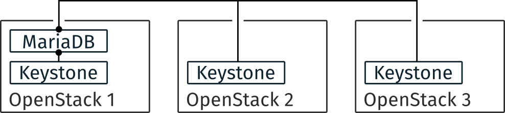
Multiple OpenStack instances deployment with a single MariaDB
Figure 1 depicts the deployment of MariaDB. MariaDB is a centralized RDBMS and thus, the Keystone backend is centralized in the first OpenStack instance. Other Keystones of other OpenStack instances refers to the backend of the first instance.
This kind of deployment comes with two possible limitations. First, a centralized RDBMS is a SPoF that makes all OpenStack instances unusable if it crashes. Second, a network disconnection of the, e.g., third OpenStack instance with the first one makes the third unusable.
Galera in multi-master replication mode and Keystone
MariaDB uses Galera Cluster as a synchronous multi-master cluster. It means that all nodes in the cluster are masters, with active-active synchronous replication, so it is possible to read or write on every node at any time. To put it simply, MariaDB Galera Cluster allows having the same database on every node thanks to synchronous replication.
To dive more into details, each time a client performs a transaction request on a node, it is processed as usual until the client issues a commit. The process is stopped and all changes made to the database in the transaction are collected in a “write-set”, along with the primary keys of the changed rows. The write-set is then broadcasted to every node with a global identifier2 to order it regarding other write-sets. The write-set finally undergoes a deterministic certification test which uses the given primary keys. It checks all transactions between the current transaction and the last successful one to determine whether the primary keys involved conflicts between each other. If the check fails, Galera rollbacks the whole transaction, and if it succeeds, Galera applies and commit the transaction on all nodes.
This is pretty efficient since it only needs one broadcast to make the replication, which means the commit does not have to wait for the responses of the other nodes. But, this means that when it fails, the entire transaction must be retried and so it may lead to more conflicts and even deadlocks.
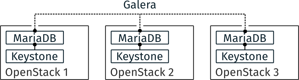
Multiple OpenStack instances deployment with Galera
Figure 3 depicts the deployment of Galera. Galera synchronizes multiple MariaDB in an active/active fashion. Thus Keystone’s backend of every OpenStack instance is replicated between all nodes, which allows reads and writes on any instances.
Regarding possible limitations, few rumors stick to Galera. First, synchronization may suffer from high latency networks. Second, contention during writes on the database may limit its scalability.
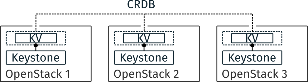
CockroachDB (abbr. CRDB) and Keystone
CockroachDB is a NewSQL database that uses the Raft protocol (an alternative version to Lamport’s Paxos consensus protocol). It uses the SQL API to enable SQL requests on every node. These requests are translated to key-value operations and -if needed- distributed across the cluster.
CockroachDB implements a single, monolithic sorted map for the keys and values stored, as seen in 4. This map is divided in ranges, which are continuous chunks of this map, with every key being in a single range, so the ranges will not overlap. Each range is then replicated (default to three replicas per range) and finally distributed across the cluster nodes.
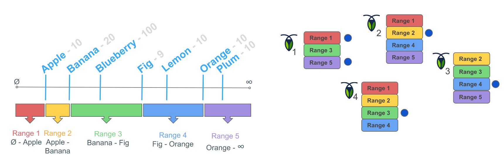
One of the replicas acts as the leaseholder, a sort of leader that coordinates all reads and writes for the range. A read only requires the leaseholder. When a write is requested, the leaseholder prepares to append it to its log, forward the request to the replicas and when the quorum is achieved, commit the change by adding it in the log. The quorum is an agreement from two out of the three replicas to make the change.
Multiple OpenStack instances deployment with CockroachDB
Figure 6 depicts the deployment of CockroachDB. In this deployment, each OpenStack instance has its Keystone. The backend is distributed through key-value stores on every OpenStack instance. Meaning, the data a Keystone is sought for is not necessarily in its local key-value store.
CockroachDB is relatively new and we know a few about its limitations, but first, CockroachDB may suffer from high network latency even during reads if the current node that gets the requests is not the leaseholder. Second, as Galera, transaction contention may dramatically slow down the overall execution. However, CockroachDB offers locality option to drive the selection of key-value stores during writes and replication. Thanks to this option it would be possible to mitigate the impact of latency by ensuring that writes happen close to the OpenStack operator.
Experiment Parameters
This section outline the two parameters considered in this study: first, the number of OpenStack instances and second, network latency. Later, the section on the locality (see, Taking into account the user locality) adds a third parameter to study heterogeneous network infrastructures.
A note about the Grid’5000 testbed and study conditions
Grid’5000 is a large-scale and versatile testbed for experiment-driven research in all areas of computer science, with a focus on parallel and distributed computing including Cloud, HPC and Big Data. The platform gives access to approximately 1000 machines grouped in 30 clusters geographically distributed in 8 sites. This study uses the ecotype cluster made of 48 nodes with each:
- CPU: Intel Xeon E5-2630L v4 Broadwell 1.80GHz (2 CPUs/node, 10 cores/CPU)
- Memory: 128 GB
- Network: - eth0/eno1, Ethernet, configured rate: 10 Gbps, model: Intel
82599ES 10-Gigabit SFI/SFP+ Network Connection, driver: ixgbe
- eth1/eno2, Ethernet, configured rate: 10 Gbps, model: Intel 82599ES 10-Gigabit SFI/SFP+ Network Connection, driver: ixgbe
The deployment of OpenStack relies on devstack stable/pike and uses default parameter for Keystone (e.g., SQL backend, fernet token, …). Juice deploys a docker version of RDBMS and tweaks a little bit devstack to ensure Keystone connects to the right RDBMS container. Note that devstack (and OpenStack) does not support CockroachDB. We published a post a few months ago about the support of CockroachDB in Keystone. Note also that RDBMS are stored directly on the memory.
Number of OpenStack instances
The OpenStack size (see, lst. 2) defines the number of OpenStack
instances deployed for an experiment. It varies between 3, 9 and
45. A value of 3, means Juice deploys OpenStack on three different
nodes, 9 on nine different nodes, … The value of 45 comes from
the maximum number of nodes available on the ecotype Grid’5000
cluster, but Juice is not limited to.
OSS = [ 3, 9, 45 ]
Experiments that test the impact of the number of OpenStack instances (see, Number of OpenStack instances impact) consider a LAN link between each OpenStack instances.
Delay
The delay (see, lst. 3) defines the network latency between
two OpenStack instances. It is expressed in terms of half the
Round-Trip Times, (i.e., a value of 50 stands for 100 ms of RTT,
150 is 300 ms of RTT). The 0 value stands for LAN speed which is
approximately 0.08 ms of RTT on the ecotype Grid’5000 cluster (10 Gbps
card).
DELAYS = [ 0, 50, 150 ]
Juice applies theses network latencies with tc netem. Note that
juice applies tc rules on network interfaces dedicated to the RDBMS
communications. Thus, metrics collection and other network
communication are not limited.
Experiments that test the impact of the network latency (see, Delay impact) are done with 9 OpenStack instances. They make the delay varies by applying traffic shaping homogeneously between the 9 OpenStack instances.
Load: Rally Scenarios
Juice uses Rally, a testing benchmarking tool for OpenStack, to evaluate how OpenStack control plane behaves at scale. This section describes Rally scenarios considered in this study. The description includes the ratio of reads and writes performed on the database. For a transactional (OLTP) database, depending on the reads/writes ratio, it could be better to choose one replication strategy to another (i.e., replicate records on all of your nodes or not).
A typical Rally execution
A Rally executes its load on one instance of OpenStack. Two variables
configure the execution of a Rally scenario: the times which is the
number of iteration execution performed for a scenario, and
concurrency which is the number of parallel iteration execution.
Thus, a scenario with times of 100 runs one hundred iterations of
the scenario by a constant load on the OpenStack instance. A
concurrency of 10 specifies that ten users concurrently achieve the
one hundred iterations. The execution output of such a scenario may
look like this:
Task 19b09a0b-7aec-4353-b215-8d5b23706cd7 | ITER: 1 START
Task 19b09a0b-7aec-4353-b215-8d5b23706cd7 | ITER: 2 START
Task 19b09a0b-7aec-4353-b215-8d5b23706cd7 | ITER: 4 START
Task 19b09a0b-7aec-4353-b215-8d5b23706cd7 | ITER: 3 START
Task 19b09a0b-7aec-4353-b215-8d5b23706cd7 | ITER: 5 START
Task 19b09a0b-7aec-4353-b215-8d5b23706cd7 | ITER: 6 START
Task 19b09a0b-7aec-4353-b215-8d5b23706cd7 | ITER: 8 START
Task 19b09a0b-7aec-4353-b215-8d5b23706cd7 | ITER: 7 START
Task 19b09a0b-7aec-4353-b215-8d5b23706cd7 | ITER: 9 START
Task 19b09a0b-7aec-4353-b215-8d5b23706cd7 | ITER: 10 START
Task 19b09a0b-7aec-4353-b215-8d5b23706cd7 | ITER: 4 END
Task 19b09a0b-7aec-4353-b215-8d5b23706cd7 | ITER: 11 START
Task 19b09a0b-7aec-4353-b215-8d5b23706cd7 | ITER: 3 END
Task 19b09a0b-7aec-4353-b215-8d5b23706cd7 | ITER: 12 START
...
Task 19b09a0b-7aec-4353-b215-8d5b23706cd7 | ITER: 100 END
Low and high load
The juice tool runs two kinds of load: low and high. The low load starts one Rally instance on only one OpenStack instance. The high load starts as many Rally instances as OpenStack instances.
The high load is named as such because it generates a lot of requests
and thus, a lot of contention on distributed RDBMS. The case of 45
Rally instances with a concurrency of 10 and times of 100 charges
450 constant transactions on the RDBMS up until getting to 4,500
iteration.
List of Rally scenarios
Here is the complete list of rally scenarios considered in this study. Values inside the parentheses refer to the percent of reads versus the percent of writes on the RDBMS. More information about each scenario is available in the appendix (see, Detailed Rally scenarios).
- keystone/authenticate-user-and-validate-token (96.46, 3.54): Authenticate and validate a Keystone token.
- keystone/create-add-and-list-user-roles (96.22, 3.78): Create a user role, add it and list user roles for given user.
- keystone/create-and-list-tenants (92.12, 7.88): Create a Keystone tenant with random name and list all tenants.
- keystone/get-entities (91.9, 8.1): Get instance of a tenant, user, role and service by id’s. An ephemeral tenant, user, and role are each created. By default, fetches the ’keystone’ service.
- keystone/create-user-update-password (89.79, 10.21): Create a Keystone user and update her password.
- keystone/create-user-set-enabled-and-delete (91.07, 8.93): Create a Keystone user, enable or disable it, and delete it.
- keystone/create-and-list-users (92.05, 7.95): Create a Keystone user with random name and list all users.
A note about gauging the %reads/%writes ratio
The %reads/%writes ratio is computed on MariaDB. The gauging code
reads values of status variables Com_xxx that provide statement
counts over all connections (with xxx stands for SELECT, DELETE,
INSERT, UPDATE, REPLACE statements). The SQL query that does
this job is available in listing 4 and returns the
total number of reads and writes since the database started. Juice
executes that SQL query before and after the execution of one Rally
scenario. After and before values are then subtracted to compute the
number of reads and writes performed during the scenario and finally,
compared to compute the ratio.
SELECT
  SUM(IF(variable_name = 'Com_select', variable_value, 0))
     AS `Total reads`,
  SUM(IF(variable_name IN ('Com_delete',
                           'Com_insert',
                           'Com_update',
                           'Com_replace'), variable_value, 0))
     AS `Total writes`
FROM  information_schema.GLOBAL_STATUS;
Note that %reads/%writes may be a little bit more in favor of reads
than what it is presented here because the following also takes into
account the creation/deletion of the Rally context. A basic Rally
context for a Keystone scenario is {"admin_cleanup@openstack":
["keystone"]}. Not sure what does this context do exactly though,
maybe it only creates an admin user…
The Juice implementation for this gauging is available on GitHub at experiments/read-write-ratio.py.
Extract, Reify and Query Rally Experiments
The execution of a Rally scenario (such as those seen in the previous section – see Load: Rally Scenarios) produces a JSON file. The JSON file contains a list of entries: one for each iteration of the scenario. An entry then retains the time (in seconds) it takes to complete all Keystone operations involved in the Rally scenario.
This section provides python facilities to extract and query Rally results for later analyses. Someone interested by the results and not by the process to compute them may skip this section and jump to the next one (see, Number of OpenStack instances impact).
An archive with results of all experiments in this study is available
at https://todo:exp-url. It contains general metrics collected over the
experiments time such as the CPU/RAM consumption, network
communications (all stored in a influxdb), plus Rally JSON result
files. Let’s assume the XPS_PATH variable references the path to the
extracted archive. Listing 5 defines accessors for all
Rally JSON result files thanks to the glob python module. The glob
module finds all paths that match specified UNIX patterns.
XP_PATHS = './ecotype-exp-backoff/'
MARIADB_XP_PATHS = glob.glob(XP_PATHS + 'mariadb-*/rally_home/*.json')
GALERA_XP_PATHS = glob.glob(XP_PATHS + 'galera-*/rally_home/*.json')
CRDB_XP_PATHS = glob.glob(XP_PATHS + 'cockroachdb-*/rally_home/*.json')
From Json files to Python Objects
A data class XP retains data of one experiment (i.e., the name of
the Rally scenario, name of database technology, … – see l.
3 to 10 of listing 6
for the complete list). Reefing experiment data in a Python object
helps for the later analyses. Indeed, a Python object makes it easier
to filter, sort, map, … experiments.
 1: @dataclass(frozen=True)
 2: class XP:
 3:     scenario: str             # Rally scenario name
 4:     rdbms: str                # Name of the RDBMS (e,g, cockcroachdb, galera)
 5:     filepath: str             # Filepath of the JSON file
 6:     oss: int                  # Number of OpenStack instances
 7:     delay: int                # Delay between nodes
 8:     high: bool                # Experiment performed during a high or light load
 9:     success: float            # Success rate (e.g., 1.0)
10:     dataframe: pd.DataFrame   # Results in a pandas 2d DataFrame
11:
12:
The XP data class comes with the make_xp function (see, lst.
7). It produces an XP object from an experiment file path
(i.e., Rally JSON file). Especially, it uses the python objectpath
module that provides a DSL to query JSON documents (à la XPath) and
extract only interesting data.
 1: def make_xp(rally_path: str) -> XP:
 2:     # Find XP name in the `rally_path`
 3:     RE_XP = r'(?:mariadb|galera|cockroachdb)-[a-zA-Z0-9\-]+'
 4:     # Find XP params in the `rally_path` (e.g., rdbms, number of OS instances, delay, ...)
 5:     RE_XP_PARAMS = r'(?P<db>[a-z]+)-(?P<oss>[0-9]+)-(?P<delay>[0-9]+)-(?P<zones>[Z0-9]{6})-(?P<high>[TF]).*'
 6:     # JSON path to the rally scenario's name
 7:     JPATH_SCN = '$.tasks[0].subtasks[0].title'
 8:
 9:     with open(rally_path) as rally_json:
10:         rally_values = objectpath.Tree(json.load(rally_json))
11:         xp_info = re.match(RE_XP_PARAMS, re.findall(RE_XP, rally_path)[0]).groupdict()
12:         success = success_rate(rally_values)
13:         return XP(
14:             scenario = rally_values.execute(JPATH_SCN),
15:             filepath = rally_path,
16:             rdbms = xp_info.get('db'),
17:             oss = int(xp_info.get('oss')),
18:             delay = int(xp_info.get('delay')),
19:             success = success,
20:             high = True if xp_info.get('high') is 'T' else False,
21:             dataframe = dataframe_per_operations(rally_values)) if success else None
The dataframe_per_operations (see l. 21) is a function
that transforms Rally JSON results in a pandas DataFrame for result analyses.
The next section will says more on this. Right now, focus on make_xp. With
make_xp, transforming all Rally JSONs into XP objects is as simple as
mapping over experiment paths (see lst. 8).
XPS = seq(MARIADB_XP_PATHS + GALERA_XP_PATHS + CRDB_XP_PATHS).truth_map(make_xp)
This study also comes with a bunch of predicates in its toolbelt that
ease the filtering and sorting of experiments. For instance, a
function def is_crdb(xp: XP) -> bool only keeps CockroachDB experiments. Likewise,
def xp_csize_rtt_b_scn_order(xp: XP) -> str returns a comparable value to sort experiments. The
complete list of predicates is available in the source of this study.
Query Rally results
The Rally JSON file contains values that give the scenario completion
time per keystone operations at a certain Rally run. These values must
be analyzed to evaluate which backend best suits an OpenStack for the
edge. And a good python module for data analysis is Pandas. Thus, the
function dataframe_per_operations (see lst.
9 – part of make_xp) takes the Rally
JSON and returns a Pandas DataFrame.
# Json path to the completion time series
JPATH_SERIES = '$.tasks[0].subtasks[0].workloads[0].data[len(@.error) is 0].atomic_actions'
def dataframe_per_operations(rally_values: objectpath.Tree) -> pd.DataFrame:
    "Makes a 2d pd.DataFrame of completion time per keystone operations."
    df = pd.DataFrame.from_items(
        items=(seq(rally_values.execute(JPATH_SERIES))
               .flatten()
               .group_by(itemgetter('name'))
               .on_value_domap(lambda it: it['finished_at'] - it['started_at'])))
    return df
The DataFrame is a table that lists all the completion times in
seconds for a specific Rally scenario. A column references a Keystone
operations and row labels (index) references the Rally run.
Listing 10 is an example of the DataFrame for
the “Create and List Tenants” Rally scenario with 9 nodes in the
CockroachDB cluster and a LAN delay between each node. The
lambda line
15 takes the DataFrame and transforms it to add a
“Total” column. Table 1 presents the output of this
DataFrame.
 1: CRDB_CLTENANTS = (XPS
 2:     # Keep xps for Keystone.create_and_list_tenants Rally scenario
 3:     .filter(is_keystone_scn('create_and_list_tenants'))
 4:     # Keep xps for 9 OpenStack instances
 5:     .filter(when_oss(9))
 6:     # Keep xps for CockroachDB backend
 7:     .filter(is_crdb)
 8:     # Keep xps for LAN delay
 9:     .filter(when_delay(0))
10:     # Keep xps for light load mode
11:     .filter(compose(not_, is_high))
12:     # Get dataframe in xp
13:     .map(attrgetter('dataframe'))
14:     # Add a Total column
15:     .map(lambda df: df.assign(Total=df.sum(axis=1)))
16:     .head())
| Iter | keystone_v3.create_project |
keystone_v3.list_projects |
Total |
|---|---|---|---|
| 0 | 0.134 | 0.023 | 0.157 |
| 1 | 0.127 | 0.025 | 0.152 |
| 2 | 0.129 | 0.024 | 0.153 |
| 3 | 0.134 | 0.023 | 0.157 |
| 4 | 0.132 | 0.024 | 0.156 |
| 5 | 0.132 | 0.025 | 0.157 |
| 6 | 0.126 | 0.024 | 0.150 |
| 7 | 0.126 | 0.026 | 0.153 |
| 8 | 0.131 | 0.025 | 0.156 |
| 9 | 0.130 | 0.025 | 0.155 |
A pandas DataFrame presents the benefits of efficiently computing a
wide range of analyses. As an example, the listing
11 computes the number of Rally runs (i.e.,
count), mean and standard deviation (i.e., mean, std), the
fastest and longest completion time (i.e., min, max), and the
25th, 50th and 75th percentiles (i.e., 25%, 50%, 75%). The
transpose method transposes row labels (index) and columns. Table
2 presents the output of the analysis.
CRDB_CLTENANTS_ANALYSIS = CRDB_CLTENANTS.describe().transpose()
| Operations | count | mean | std | min | 25% | 50% | 75% | max |
|---|---|---|---|---|---|---|---|---|
keystone_v3.create_project |
10.000 | 0.130 | 0.003 | 0.126 | 0.128 | 0.131 | 0.132 | 0.134 |
keystone_v3.list_projects |
10.000 | 0.024 | 0.001 | 0.023 | 0.024 | 0.024 | 0.025 | 0.026 |
| Total | 10.000 | 0.155 | 0.003 | 0.150 | 0.153 | 0.155 | 0.157 | 0.157 |
Experiment Analysis
This section presents the results of experiments and their analysis. To avoid lengths of graphics in this report, only a short version of the results are presented. The entirety of the results, that is, median time for each Rally scenarios and cumulative distribution functions for each scenarios, are located in the appendix (see, Detailed experiments results).
The short results focus on two Rally scenarios. First, authenticate and validate a keystone token (%reads: 96.46, %writes: 3.54), which represents more than 95% of what is actually done on a running Keystone. Second, create user and update password for that user (%reads: 89.79, %writes: 10.21), which gets the highest rate of writes and thus, the most likely to produce contention on the RDBMS.
In next result plots, the λ Greek letter stands for the failure rate and σ for the standard deviation.
Number of OpenStack instances impact
This test evaluates how the completion time of Rally Keystone’s
scenarios varies, depending on the RDBMS and the number of OpenStack
instances. It measure the capacity of a RDBMS to handle lot of
connections and requests. In this test, the number of OpenStack
instances varies between 3, 9 and 45 and a LAN link
inter-connects instances. As explain in the OpenStack at the Edge
section, the deployment of the database depends on the RDBMS. With
MariaDB, one instance of OpenStack contains the database, and others
connect to that one. For Galera and CockroachDB, every OpenStack
contains an instance of the RDBMS.
For these experiments, Juice deployed database together with OpenStack instances and plays Rally scenarios listed in section List of Rally scenarios. Juice runs Rally scenarios under both light and high load. Results are presented in the two next subsections. The Juice implementation for these experiments is available on GitHub at experiments/cluster-size-impact.py.
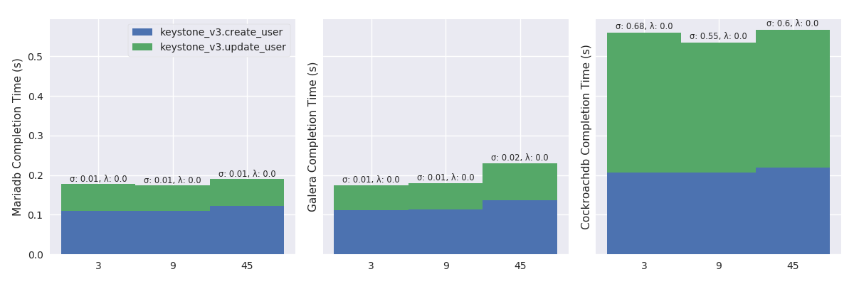
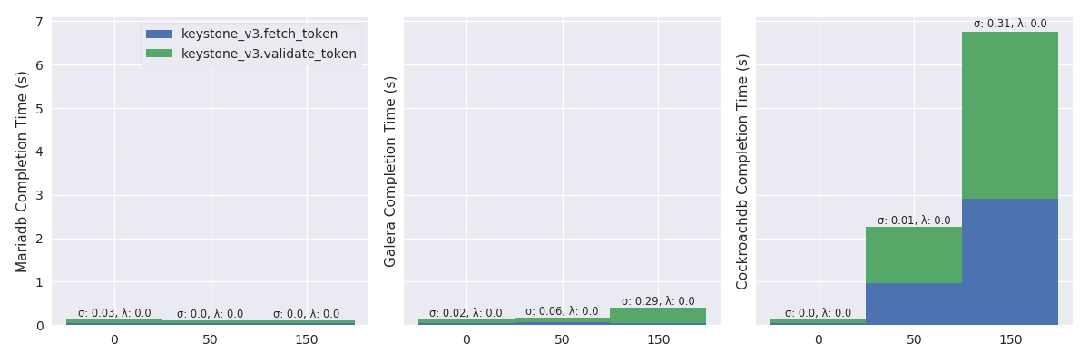
Authenticate and validate a Keystone token (%r: 96.46, %w: 3.54)
Figure 7 plots the mean completion time (in
second) of Keystone authenticate and validate a keystone token (%r:
96.46, %w: 3.54) scenario in a light Rally mode. The plot displays
results in three tiles. The first tile shows completion time with the
centralized MariaDB, second tile with the replicated Galera and, third
tile with the global CockroachDB. A tile presents results with stacked
bar charts. A bar depicts the total completion time for a specific
number of OpenStack instances (i.e., 3, 9 and 45) and stacks
completion times of each Keystone operations. The figure shows that
the trend is similar for the three RDBMS, to the advantage of the
centralized MariaDB, followed by Galera and then CockroachDB.
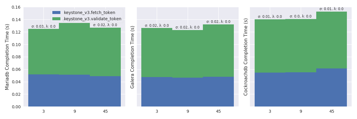
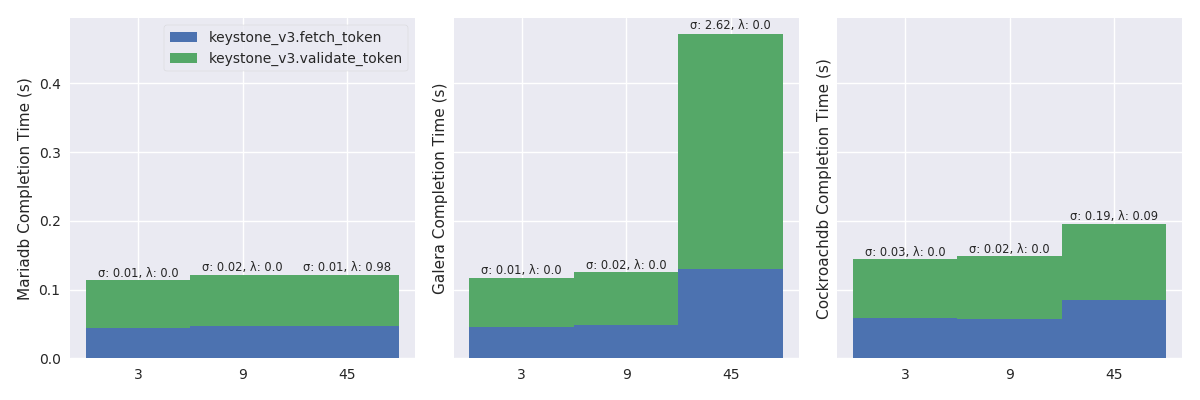
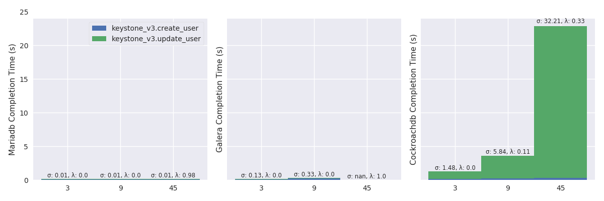
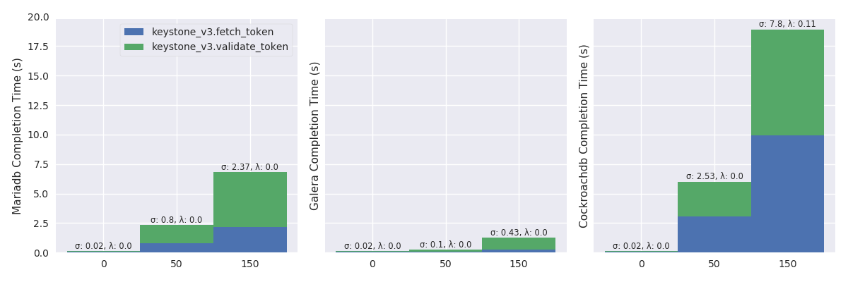
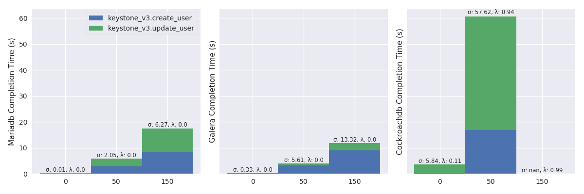
Figure 8 shows that putting pressure using the high load has strong effects on MariaDB and Galera while CockroachDB well handles it. With 45 OpenStack instances, the failure rate of MariaDB rises from 0 to 98 percent (i.e., λ: 0.98) and, the mean completion time of Galera rises from 120 to 475 milliseconds (namely, an increased by a factor of 4).
TODO:explenation (look at MariaDB log).
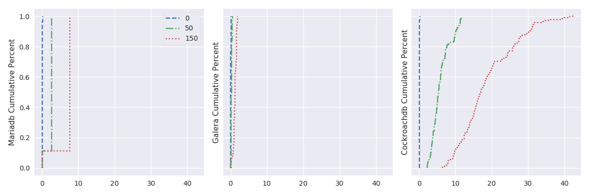
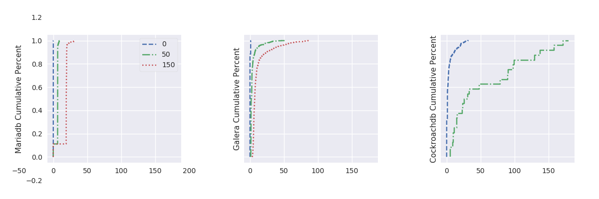
TODO:explenation (look at Galera log). Plotting the cumulative distribution function (i.e., the probability that the scenario complete in less or equal than a certain time – see, fig. 9) shows that, with 45 OpenStack instances, more than 95% of the results should complete in a reasonable time, but the lasts 5% may take a really long time to complete (here, up to 30 second).
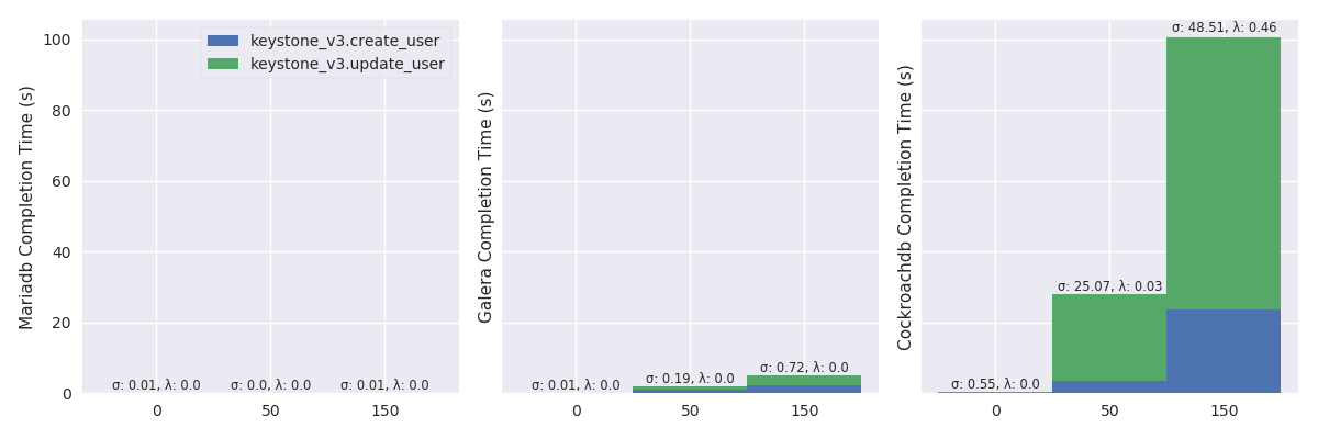
Create a user and update her password (%r: 89.79, %w: 10.21)
Figure 7 plots the mean completion time (in second) of Keystone Create a user and update her password (%r: 89.79, %w: 10.21) scenario in a light Rally mode.
High mode
CDF
Scale outline
TODO:
| RDBMS | Scale | Note |
|---|---|---|
| MariaDB | 😺️ | |
| Galera | 😾️ | |
| CockroachDB | 😺 |
Delay impact
In this test, the size of the database cluster is 9 and the delay varies between LAN, 100 and 300 ms of RTT. The test evaluates how the completion time of Rally scenarios varies, depending of RTT between nodes of the swarm.
- TODO: describe the experimentation protocol
- TODO: Link the github juice code
Authenticate and validate a Keystone token (%r: 96.46, %w: 3.54)
Auth. Light Mode
High Mode
CDF
Create a user and update her password (%r: 89.79, %w: 10.21)
Create Light Mode
High Mode
CDF
Network delay outline
TODO:
| RDBMS | Network Delay | Note |
|---|---|---|
| MariaDB | 😺 | |
| Galera | 😺 reads, 😾 writes | |
| CockroachDB | 😾 |
Taking into account the user locality
A homogeneous delay is sometimes needed but does not map to the edge reality where some nodes are closed and other are far. To simulate such heterogeneous network infrastructure …
ZONES = [ ('Z1', 'Z2', 'Z3'), ('Z1', 'Z1', 'Z3'), ('Z1', 'Z1', 'Z1') ]
zones: Tuple[str,str,str] = ('Z1', 'Z1', 'Z1') # Replication Zones
zones = tuple([xp_info.get('zones')[x:x+2] for x in range(0, len(xp_info.get('zones')), 2)]),
zones_plot = frame_plot(ZONES)
Delay distribution: uniform & hierarchical
This study considers two kinds of OpenStack instances deployments.
This first one, called uniform, defines a uniform distribution of
the network latency between OpenStack instances. For instance, 300
ms of RTT between all the 9 OpenStack instances. The second
deployment, called hierarchical, maps to a more realistic view, like
in cloud computing, with groups of OpenStack instances connected
through a low latency network (e.g., 3 OpenStack instances per
group deployed in the same country, and accessible within 20 ms of
RTT). And high latency network between groups (e.g. 150 ms of RTT
between groups deployed in different countries).
XPS_ZONES = (XPS
    # We are only interested in results with 9 OpenStack instances
    .filter(when_oss(9))
    .filter(when_delay(10))
    .filter(compose(not_, is_high))
    # .filter(is_keystone_scn('get_entities'))
    # .filter(is_crdb)
    # Also, remove values greater than the 95th percentile
    .map(lambda xp: xp.set_dataframe(filter_percentile(.95, xp.dataframe)))
)
CDF
Locality outline
| RDBMS | Network Delay w/ Locality | Note |
|---|---|---|
| MariaDB | 😺 | |
| Galera | 😺 reads, 😾 writes | |
| CockroachDB | 😺 |
Experiments Outline
TODO:
| RDBMS | Scale | Network Delay | Note |
|---|---|---|---|
| MariaDB | 😺 | 😺 | |
| Galera | 😾 | 😺 reads, 😾 writes | |
| CockroachDB | 😺 | 😺 with locality, 😾 otherwise |
TODO: General purpose support of locality
Appendix
Detailed experiments results
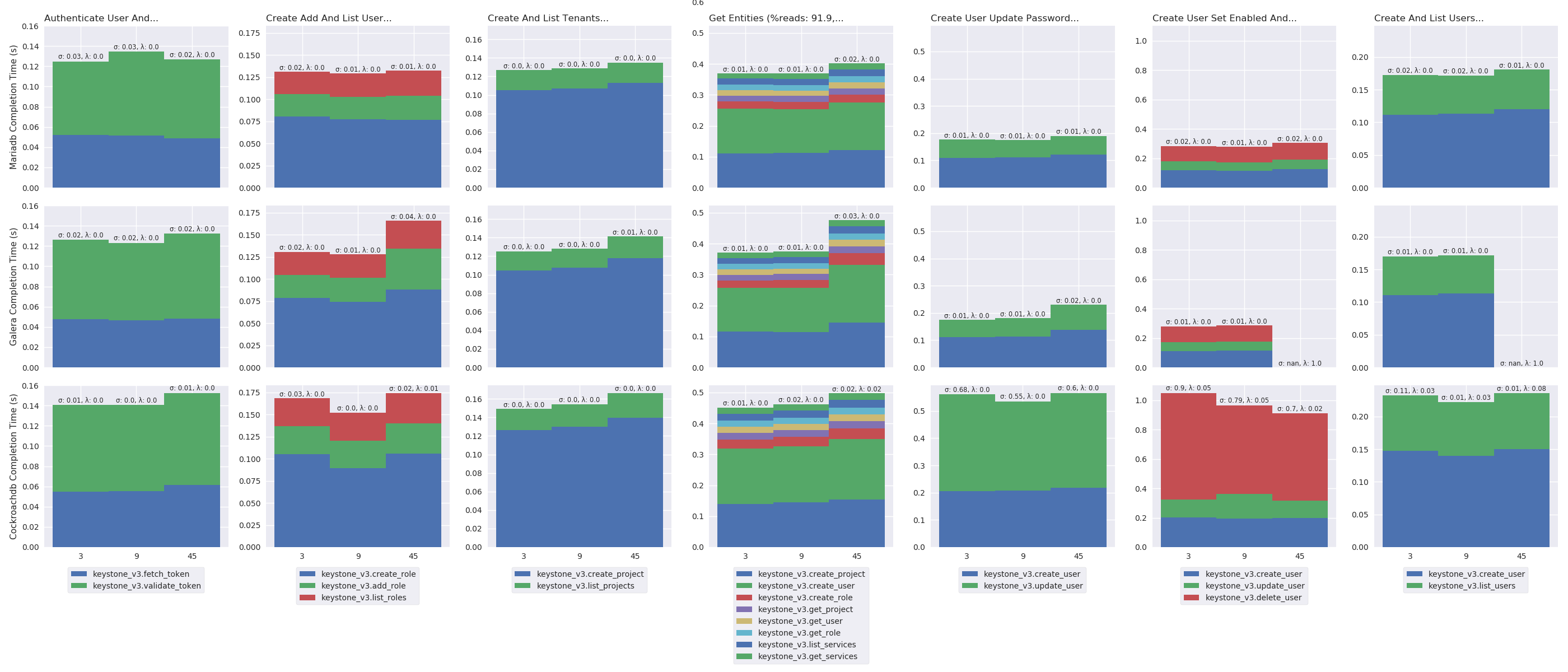
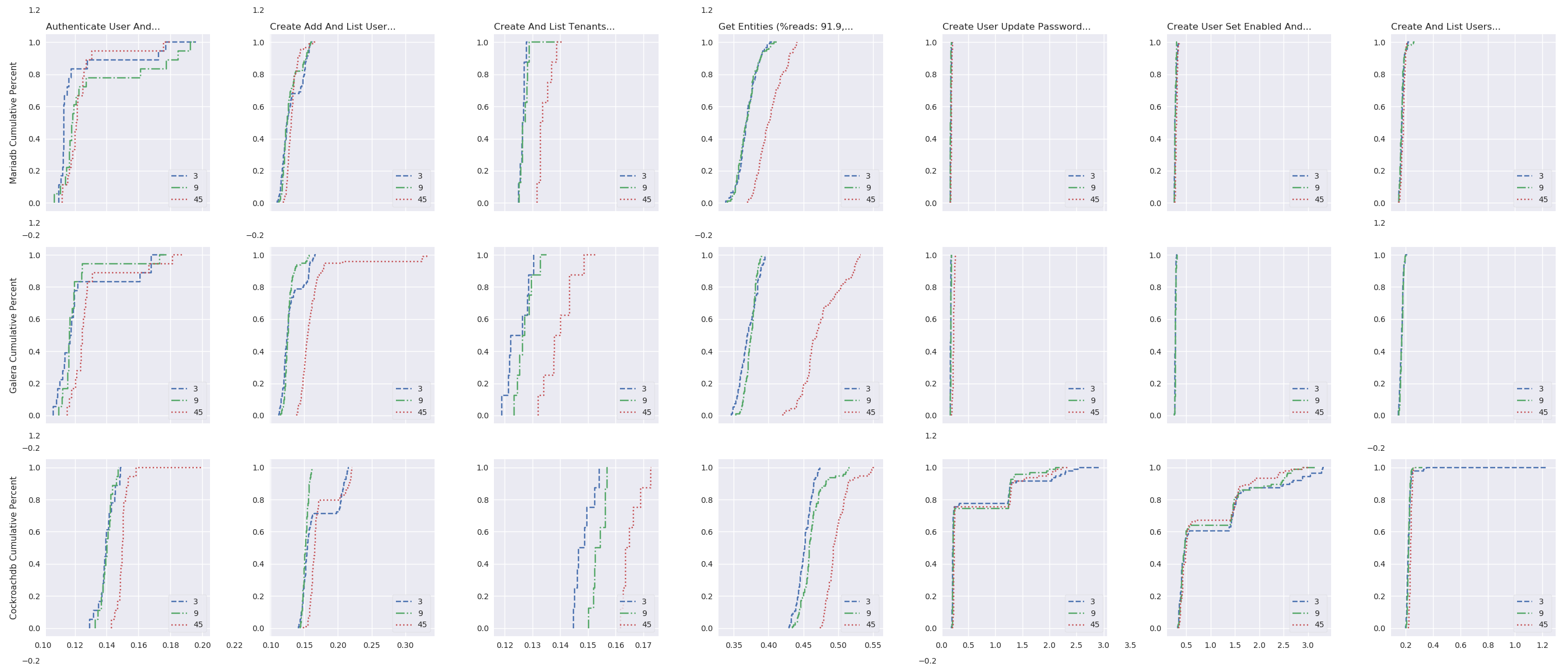
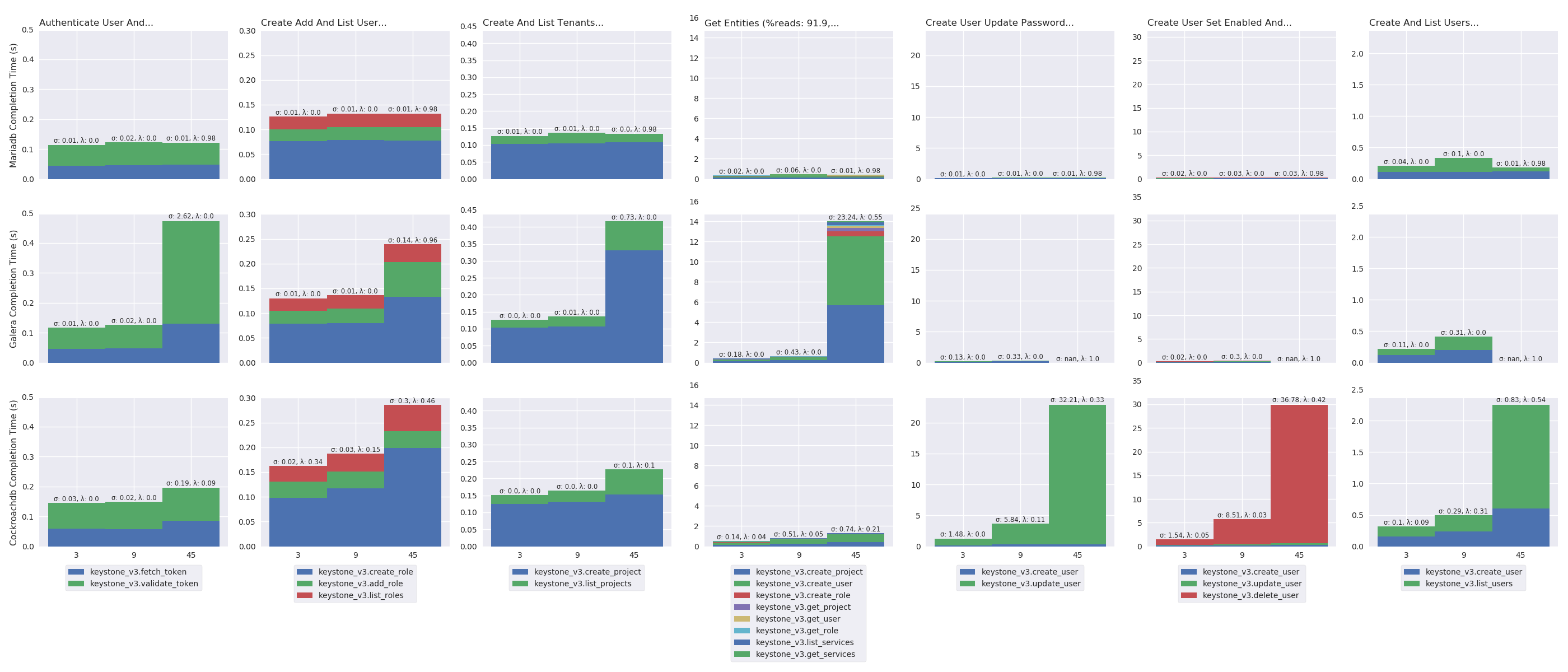
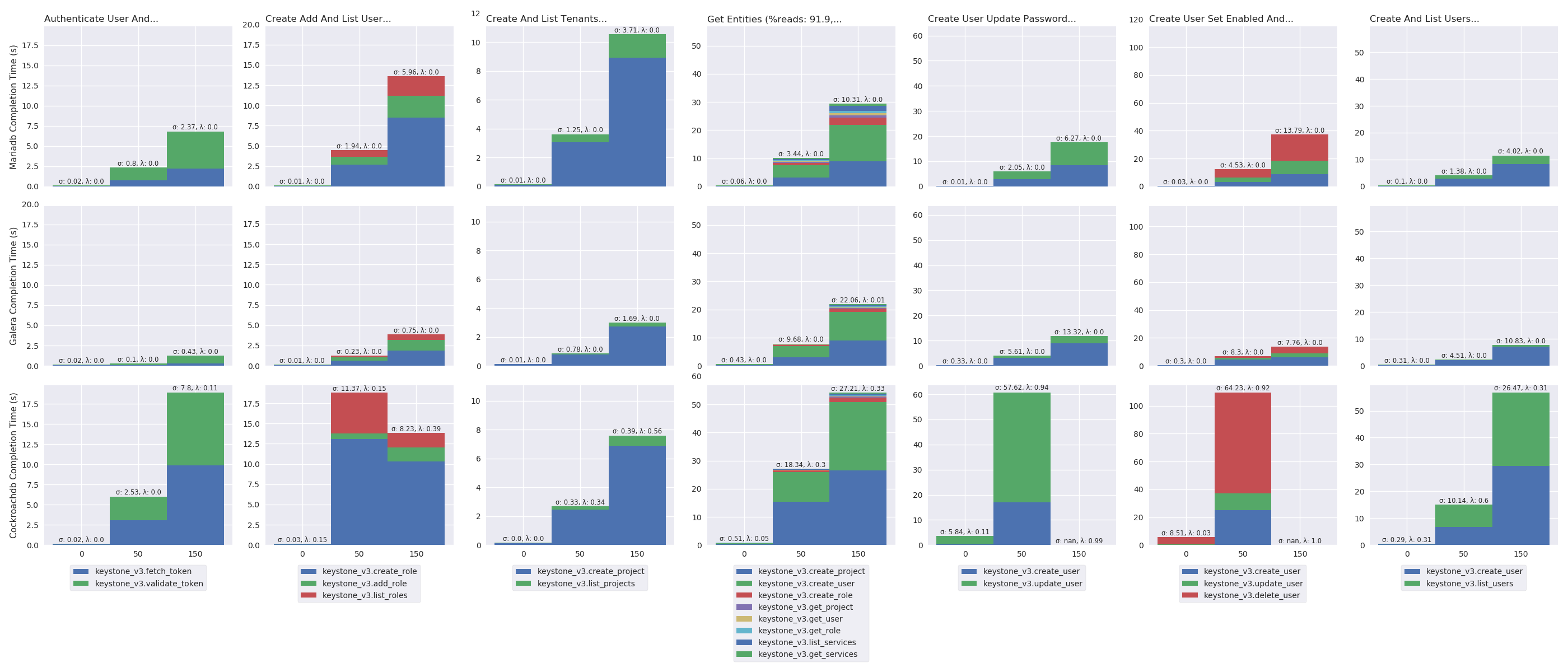
Listing 15 computes the mean completion time (in
second) of Rally scenarios in a light mode and plots the results in
figure 19. In the following figure, columns presents
results of a specific scenario: the first column presents results for
Authenticate User and Validate Token, the second for Create Add and
List User Role. Rows present results with a specific RDBMS: first row
presents results for MariaDB, second for Galera and third for
CockroachDB. The figure presents results with stacked bar charts. A
bar presents the result for a specific number of OpenStack instances
(i.e., 3, 9 and 45) and stacks completion times of each
Keystone operations.
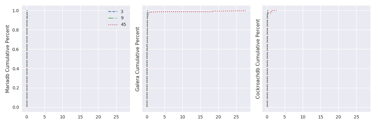
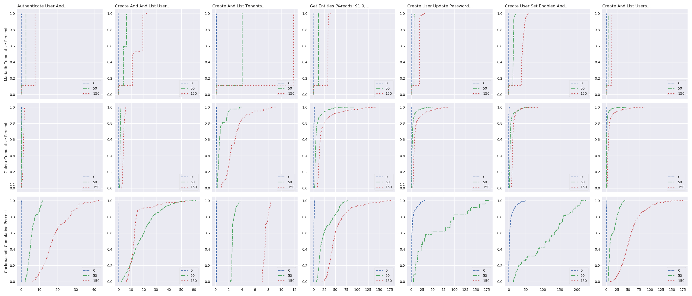
Number of OpenStack instances impact under light load
oss_plot("%s Completion Time (s)",
         series_stackedbar_plot,
         'imgs/oss-impact-light',
         (# -- Experiments selection
          XPS
          # We are only interested in results where delay is LAN
          .filter(when_delay(0))
          # remove values greater than the 95th percentile
          .map(lambda xp: xp.set_dataframe(filter_percentile(.95, xp.dataframe)))
          # Filter light load
          .filter(compose(not_, is_high))
          # Group results by scenario's name, RDBMS technology and
          # number of OpenStack instances.
           .group_by(lambda xp: (xp.scenario, xp.rdbms, xp.oss))
          # Compute the mean, std and success of the results
          .on_value_domap(lambda xp: (xp.dataframe, xp.success))
          .on_value(unpack(lambda dfs, succs: (pd.concat(dfs), np.mean(succs))))
          .on_value(unpack(lambda df, succ: (df.mean(), df.sum(axis=1).std(), succ)))
          .to_dict()))
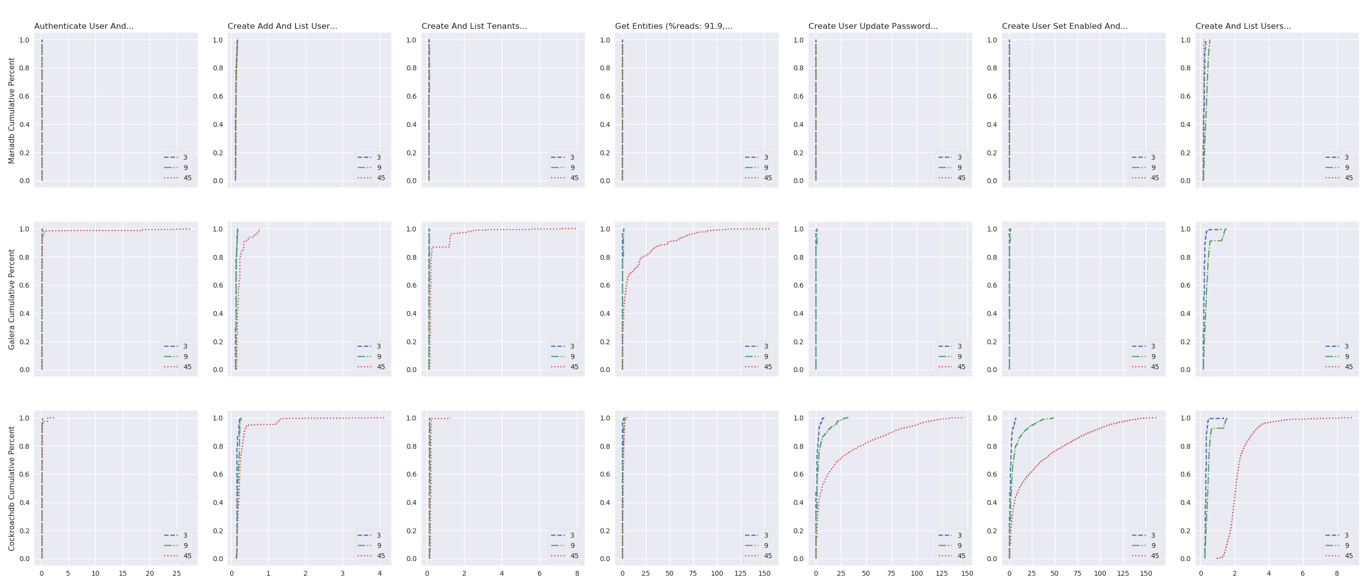
oss_plot("%s Cumulative Percent",
         series_linear_plot,
         'imgs/oss-impact-light-cdf',
         (# -- Experiments selection
          XPS
          # We are only interested in results where delay is LAN
          .filter(when_delay(0))
          # remove values greater than the 95th percentile
          .map(lambda xp: xp.set_dataframe(filter_percentile(.95, xp.dataframe)))
          # Filter light load
          .filter(compose(not_, is_high))
          # Group results by scenario's name, RDBMS technology and
          # number of OpenStack instances.
          .group_by(lambda xp: (xp.scenario, xp.rdbms, xp.oss))
          # Compute the CDF of the resuls
          .on_value_domap(attrgetter('dataframe'))
          .on_value(lambda dfs: pd.concat(dfs))
          .on_value(lambda df: df.sum(axis='columns'))
          .on_value(make_cumulative_frequency)
          .to_dict()),
         legend='all')
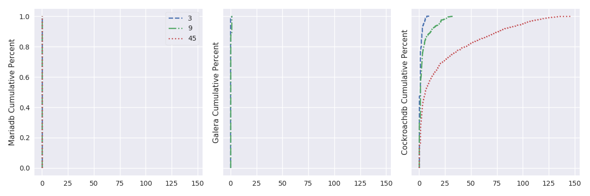
Number of OpenStack instances impact under high load
oss_plot("%s Completion Time (s)",
         series_stackedbar_plot,
         'imgs/oss-impact-high',
         (# -- Experiments selection
          XPS
          # We are only interested in results where delay is LAN
          .filter(when_delay(0))
          # remove values greater than the 95th percentile
          .map(lambda xp: xp.set_dataframe(filter_percentile(.95, xp.dataframe)))
          # Filter high load
          .filter(is_high)
          # Group results by scenario's name, RDBMS technology and
          # number of OpenStack instances.
          .group_by(lambda xp: (xp.scenario, xp.rdbms, xp.oss))
          # Compute the mean, std and success of the results
          .on_value_domap(lambda xp: (xp.dataframe, xp.success))
          .on_value(unpack(lambda dfs, succs: (pd.concat(dfs), np.mean(succs))))
          .on_value(unpack(lambda df, succ: (df.mean(), df.sum(axis=1).std(), succ)))
          .to_dict()))
oss_plot("%s Cumulative Percent",
         series_linear_plot,
         'imgs/oss-impact-high-cdf',
         (# -- Experiments selection
          XPS
          # We are only interested in results where delay is LAN
          .filter(when_delay(0))
          # remove values greater than the 95th percentile
          .map(lambda xp: xp.set_dataframe(filter_percentile(.95, xp.dataframe)))
          # Filter high load
          .filter(is_high)
          # Group results by scenario's name, RDBMS technology and
          # number of OpenStack instances.
          .group_by(lambda xp: (xp.scenario, xp.rdbms, xp.oss))
          # Compute the CDF of the resuls
          .on_value_domap(attrgetter('dataframe'))
          .on_value(lambda dfs: pd.concat(dfs))
          .on_value(lambda df: df.sum(axis='columns'))
          .on_value(make_cumulative_frequency)
          .to_dict()
         ), legend='all')
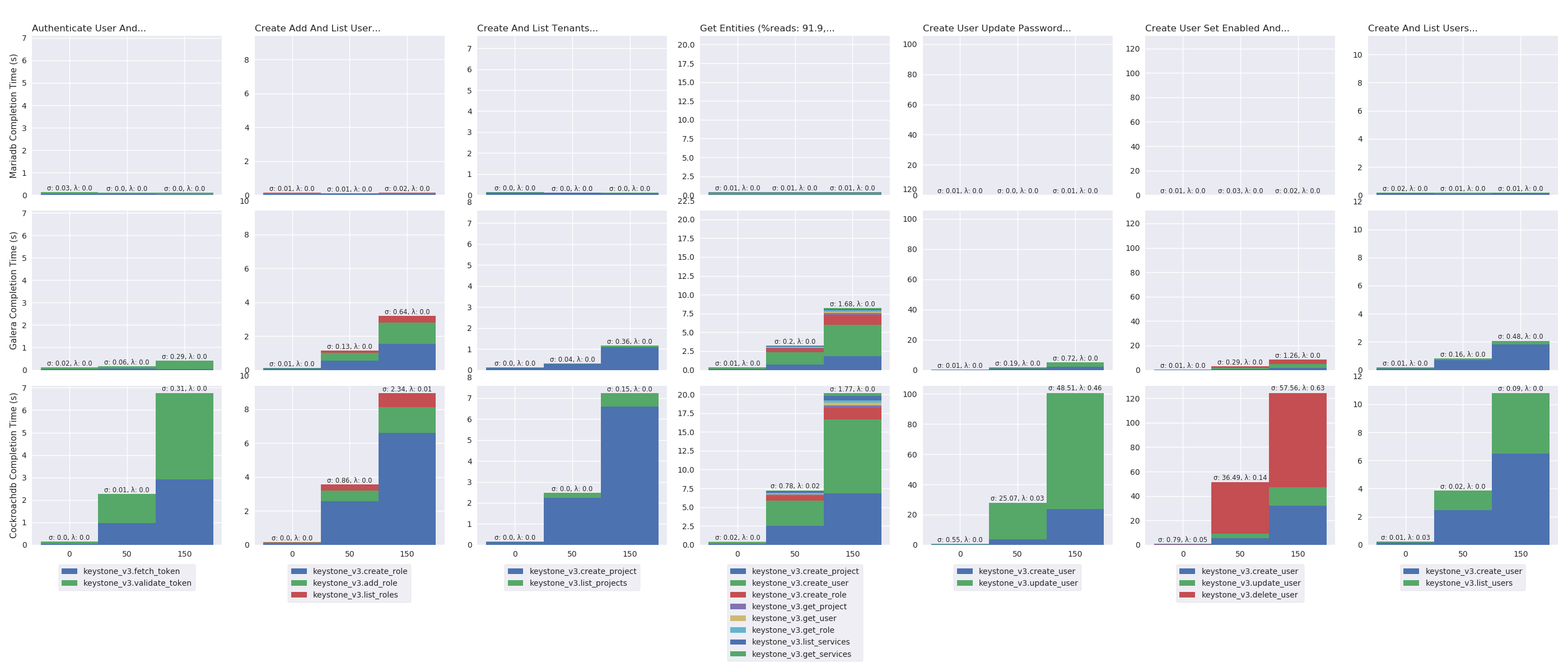
Delay impact under light load
delay_plot("%s Completion Time (s)",
           series_stackedbar_plot,
           'imgs/delay-impact-light',
           (# -- Experiments selection
            XPS
            # We are only interested in results with 9 OpenStack instances
            .filter(when_oss(9))
            .filter(compose(not_, when_delay(10)))
            # Also, remove values greater than the 95th percentile
            .map(lambda xp: xp.set_dataframe(filter_percentile(.95, xp.dataframe)))
            # Filter light load
            .filter(compose(not_, is_high))
            # Group results by scenario's name, RDBMS technology and
            # delay
            .group_by(lambda xp: (xp.scenario, xp.rdbms, xp.delay))
            # Compute the mean, std and success of the results
            .on_value_domap(lambda xp: (xp.dataframe, xp.success))
            .on_value(unpack(lambda dfs, succs: (pd.concat(dfs), np.mean(succs))))
            .on_value(unpack(lambda df, succ: (df.mean(), df.sum(axis=1).std(), succ)))
            .to_dict()
         ))
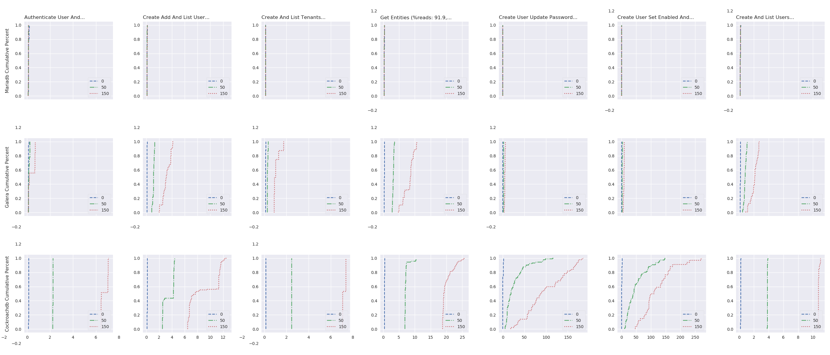
delay_plot("%s Cumulative Percent",
           series_linear_plot,
           'imgs/delay-impact-light-cdf',
           (# -- Experiments selection
            XPS
            # We are only interested in results with 9 OpenStack instances
            .filter(when_oss(9))
            .filter(compose(not_, when_delay(10)))
            # Also, remove values greater than the 95th percentile
            .map(lambda xp: xp.set_dataframe(filter_percentile(.95, xp.dataframe)))
            # Filter light load
            .filter(compose(not_, is_high))
            # Group results by scenario's name, RDBMS technology and
            # delay
            .group_by(lambda xp: (xp.scenario, xp.rdbms, xp.delay))
            # Compute the CDF
            .on_value_domap(attrgetter('dataframe'))
            .on_value(lambda dfs: pd.concat(dfs))
            .on_value(lambda df: df.sum(axis='columns'))
            .on_value(make_cumulative_frequency)
            .to_dict()
         ), legend='all')
Delay impact under high load
delay_plot("%s Completion Time (s)",
           series_stackedbar_plot,
           'imgs/delay-impact-high',
           (# -- Experiments selection
            XPS
            # We are only interested in results with 9 OpenStack instances
            .filter(when_oss(9))
            .filter(compose(not_, when_delay(10)))
            # Also, remove values greater than the 95th percentile
            .map(lambda xp: xp.set_dataframe(filter_percentile(.95, xp.dataframe)))
            # Filter high load
            .filter(is_high)
            # Group results by scenario's name, RDBMS technology and
            # delay
            .group_by(lambda xp: (xp.scenario, xp.rdbms, xp.delay))
            # Compute the mean, std and success of the results
            .on_value_domap(lambda xp: (xp.dataframe, xp.success))
            .on_value(unpack(lambda dfs, succs: (pd.concat(dfs), np.mean(succs))))
            .on_value(unpack(lambda df, succ: (df.mean(), df.sum(axis=1).std(), succ)))
            .to_dict()
         ))
delay_plot("%s Cumulative Percent",
           series_linear_plot,
           'imgs/delay-impact-high-cdf',
           (# -- Experiments selection
            XPS
            # We are only interested in results with 9 OpenStack instances
            .filter(when_oss(9))
            .filter(compose(not_, when_delay(10)))
            # Also, remove values greater than the 95th percentile
            .map(lambda xp: xp.set_dataframe(filter_percentile(.95, xp.dataframe)))
            # Filter high load
            .filter(is_high)
            # Group results by scenario's name, RDBMS technology and
            # delay
            .group_by(lambda xp: (xp.scenario, xp.rdbms, xp.delay))
            # Compute the CDF
            .on_value_domap(attrgetter('dataframe'))
            .on_value(lambda dfs: pd.concat(dfs))
            .on_value(lambda df: df.sum(axis='columns'))
            .on_value(make_cumulative_frequency)
            .to_dict()
         ), legend='all')
Take into account the client locality
Detailed Rally scenarios
keystone/authenticate-user-and-validate-token
Description: authenticate and validate a keystone token.
Definition Code: samples/tasks/scenarios/keystone/authenticate-user-and-validate-token
Source Code: rally_openstack.scenarios.keystone.basic.AuthenticateUserAndValidateToken
List of keystone functionalities:
- keystone_v3.fetch_token
- keystone_v3.validate_token
%Reads/%Writes: 96.46/3.54
Number of runs: 20
keystone/create-add-and-list-user-roles
Description: create user role, add it and list user roles for given user.
Definition Code: samples/tasks/scenarios/keystone/create-add-and-list-user-roles
Source Code: rally_openstack.scenarios.keystone.basic.CreateAddAndListUserRoles
List of keystone functionalities:
- keystone_v3.create_role
- keystone_v3.add_role
- keystone_v3.list_roles
%Reads/%Writes: 96.22/3.78
Number of runs: 100
keystone/create-and-list-tenants
Description: create a keystone tenant with random name and list all tenants.
Definition Code: samples/tasks/scenarios/keystone/create-and-list-tenants
Source Code: rally_openstack.scenarios.keystone.basic.CreateAndListTenants
List of keystone functionalities:
- keystone_v3.create_project
- keystone_v3.list_projects
%Reads/%Writes: 92.12/7.88
Number of runs: 10
keystone/get-entities
Description: get instance of a tenant, user, role and service by id’s. An ephemeral tenant, user, and role are each created. By default, fetches the ’keystone’ service.
List of keystone functionalities:
- keystone_v3.create_project
- keystone_v3.create_user
- keystone_v3.create_role
- keystone_v3.list_roles
- keystone_v3.add_role
- keystone_v3.get_project
- keystone_v3.get_user
- keystone_v3.get_role
- keystone_v3.list_services
- keystone_v3.get_services
%Reads/%Writes: 91.9/8.1
Definition Code: samples/tasks/scenarios/keystone/get-entities
Source Code: rally_openstack.scenarios.keystone.basic.GetEntities
Number of runs: 100
keystone/create-user-update-password
Description: create user and update password for that user.
List of keystone functionalities:
- keystone_v3.create_user
- keystone_v3.update_user
%Reads/%Writes: 89.79/10.21
Definition Code: samples/tasks/scenarios/keystone/create-user-update-password
Source Code: rally_openstack.scenarios.keystone.basic.CreateUserUpdatePassword
Number of runs: 100
keystone/create-user-set-enabled-and-delete
Description: create a keystone user, enable or disable it, and delete it.
List of keystone functionalities:
- keystone_v3.create_user
- keystone_v3.update_user
- keystone_v3.delete_user
%Reads/%Writes: 91.07/8.93
Definition Code: samples/tasks/scenarios/keystone/create-user-set-enabled-and-delete
Source Code: rally_openstack.scenarios.keystone.basic.CreateUserSetEnabledAndDelete
Number of runs: 100
keystone/create-and-list-users
Description: create a keystone user with random name and list all users.
List of keystone functionalities:
- keystone_v3.create_user
- keystone_v3.list_users
%Reads/%Writes: 92.05/7.95
Definition Code: samples/tasks/scenarios/keystone/create-and-list-users
Source Code: rally_openstack.scenarios.keystone.basic.CreateAndListUsers.
Number of runs: 100
Footnotes
1 Here we present two deployment alternatives. But there are several others such as multiple regions, CellV2 and federation deployment.
2 TODO(Comment on global identifier): general way to implement this is vector clock + causal broadcast (i.e., costly operation). Actually, galera do not tell how it implement this but say that it uses a clock that may differ of 1 second from one peer to another. This means that two concurrent transactions, on two different peers, done during the same second may end with the same id. Henceforth, Galera do not ensure first order commit and inconsistency may arises.
Comments
Patrick Royer
October 31st, 2018, 05.46pm
Bonjour, merci pour ce papier très bien rédigé. Je ne vois pas la version de CockroachDB utilisée, était-ce une version 2+ ?
Ronan-A. Cherrueau
November 10th, 2018, 12.04pm
Hi Patrick,
Good question, we did experiments with CockroachDB version 2.0.1. Recently, CockroachDB published version 2.1 that comes with two exciting enhancements that should change results above:
We plan to redo experiments with CockroachDB 2.1 and finish this article based on the new results. But we currently struggle to run OpenStack on top of it.
Leave a comment